* 본 포스트는 개인연구/학습 기록 용도로 작성되고 있습니다.
[Python] Long/Short Pair Trading
By MK on January 26, 2019
Long-Short 전략은 장기, 단기 보유 주식 개념과 유사하다.
Pair Trading이 어떤 주식이 저평가되어 있고 고평가되어있는지를 식별하는 것처럼 Long-Short 전략도 어느 주식이 상대적으로 저렴하고 비싼지를 식별하기 위해 Basket내 주식에 순위를 매긴다.
그런 다음 순위에 따라 상위 n개는 장기 매입하고 동일한 금액에 대해 하단 n개를 매도한다.
Pairs Trading, Long-Short의 핵심은 시장중립적이라는 것이다.
What is a Ranking Scheme?
주식 바구니에서 주식별 랭킹을 매기는 것을 의미하다. 예를 들면 가치요소, 기술지표, 가격모델 또는 모든 것의 조합이 기준이 될 수 있다.
모멘텀지표를 사용하여 추세를 따르는 주식 바구니에 순위를 매길수도 있다. 가장 높은 모멘텀을 보유한 주식은 계속 호조를 나타내며 가장 높은 순위를 얻는다. 가장 낮은 모멘텀을 가진 주식은 최악의 상황을 수행하고 가장 낮은 수익을 얻게 된다.
이 전략의 성공은 전적으로 Ranking Scheme에 달려있다.
전제조건
n(투자금액) = 1000
m(자산의 갯수) = 10
총 2p의 포지션을 보유하고 싶다고 가정해보자.
주식 랭킹을 나열하면 아래와 같다.
1,2, .. p, … m=10
다만 2p는 매도/매수 포지션이 동일하여 * 2 한 개념이다. 즉, 2p는 m보다 클 수 없다.
이런 상황에서 순위 1의 주가가 최악의 실적을 보일 것으로 예상되고 순위 m이 우수한 성과를 낼 것으로 예상될 때,
Price = n/2p
p가 5라면, 1000/(2 * 5) = 100
1~p의 주식들을 Price에 매도하고, p~m의 주식들을 Price에 매수한다.
즉 100씩 p=5개, 500을 매수/매도하게 된다.
여기서 문제는 항상 Price가 정수가 될 수 없어 모델의 부정확도의 원인이 될 수 있으며, 100 이하의 단가 종목만 거래가 가능하다.
이는 보다 자본을 증가시키거나(분자↑) 더 적은 양의 거래(분모↓)를 하는 것으로 완화할 수 있다.
사용한 라이브러리
import FinanceDataReader as fdr
fdr.__version__

import pandas as pd
import numpy as np
import statsmodels.api as sm
import scipy.stats as stats
import scipy
import matplotlib.pyplot as plt
import seaborn as sns
1. 데이터 가져오기
종목별 시세 데이터를 가져올 수 있으면 된다.
아래 코드는 FinanceDataReader를 사용할때 특정 기간내 종목별 데이터 건수가 상이하여 임시 작업한 케이스이다.
# 한국거래소 상장종목 전체
# 용도 : 코드와 종목명 가져오기
df_krx = fdr.StockListing('KRX')

# 코스피 종목 추출
# 용도 : DataReader 사용시 종목별 기간 조회 건수가 상이하다.
#        코스피 데이터 날짜를 기준으로 가져오기 위해 사용
strt_dt = '2014-01-01' # 시작일 지정
end_dt = '2018-12-31'  # 종료일 지정
kospi_df = fdr.DataReader('KS11', strt_dt,end_dt)
kospi_df.reset_index(inplace = True)
def stock_reader(kospi_df, code_list, n=0):

    if n == 0:
        n = len(code_list)

    stock_df = pd.DataFrame()
    stock_df['Date'] = kospi_df['Date']
    print("동기간 KOSPI 생성일수 : ", len(kospi_df['Date']))
    normal_cnt = 0
    err_cnt = 0
    code_nm_list = []

    for code in code_list:
        stock = df_krx[df_krx.Symbol == code]
        code_nm = list(stock.Name)[0]


        try:
            temp = fdr.DataReader(code, strt_dt, end_dt)

            # 데이터일수가 시장보다 작으면 skip(최근 상장 데이터로 판단)
            if len(temp) < len(kospi_df['Date']):
                err_cnt += 1
                print("skip : (",err_cnt,")", code, code_nm, strt_dt, end_dt, ", 건수 : ", len(temp))
                continue

            temp.reset_index(inplace = True)
            temp_df = pd.merge(temp[['Date','Close']], kospi_df[['Date']], on='Date', how='right')
            stock_df[code_nm] = temp_df.Close
            normal_cnt += 1
            code_nm_list.append(code_nm)
            print("정상 : (",normal_cnt,")", code, code_nm, strt_dt, end_dt, ", 건수 : ", len(temp), "->", len(stock_df))
        except:
            err_cnt += 1
            print("skip : (",err_cnt,")", code, code_nm, strt_dt, end_dt, ", 건수 : ", len(temp))

        if normal_cnt == n:
            print('총', n,'개 생성 설정 / ', normal_cnt, '개 생성 완료')
            break # n개 종목 생성시 종료

        # 데이터 정렬
        stock_df.sort_values('Date', ascending=True, inplace=True) # ascending=True 오름차순, False 내림차순
        # 결측치 채우기
        stock_df.fillna(method='ffill', inplace=True)

    return stock_df, code_nm_list
추출할 종목수 지정
n = 10 # 생성할 종목수 지정
df_krx_list = df_krx['Symbol'].head(n*2) # 임시로 2배까지 루프

stock_df, code_nm_list = stock_reader(kospi_df, df_krx_list, n)
동기간 KOSPI 생성일수 :  1226
정상 : ( 1 ) 001040 CJ 2014-01-01 2018-12-31 , 건수 :  1331 -> 1226
정상 : ( 2 ) 011150 CJ씨푸드 2014-01-01 2018-12-31 , 건수 :  1298 -> 1226
정상 : ( 3 ) 082740 HSD엔진 2014-01-01 2018-12-31 , 건수 :  1305 -> 1226
정상 : ( 4 ) 001390 KG케미칼 2014-01-01 2018-12-31 , 건수 :  1313 -> 1226
정상 : ( 5 ) 010060 OCI 2014-01-01 2018-12-31 , 건수 :  1434 -> 1226
정상 : ( 6 ) 002360 SH에너지화학 2014-01-01 2018-12-31 , 건수 :  1410 -> 1226
정상 : ( 7 ) 001740 SK네트웍스 2014-01-01 2018-12-31 , 건수 :  1395 -> 1226
skip : ( 1 ) 285130 SK케미칼 2014-01-01 2018-12-31 , 건수 :  264
skip : ( 2 ) 011810 STX 2014-01-01 2018-12-31 , 건수 :  916
정상 : ( 8 ) 024070 WISCOM 2014-01-01 2018-12-31 , 건수 :  1233 -> 1226
정상 : ( 9 ) 011420 갤럭시아에스엠 2014-01-01 2018-12-31 , 건수 :  1298 -> 1226
skip : ( 3 ) 267290 경동도시가스 2014-01-01 2018-12-31 , 건수 :  402
정상 : ( 10 ) 002240 고려제강 2014-01-01 2018-12-31 , 건수 :  1258 -> 1226
총 10 개 생성 설정 /  10 개 생성 완료
stock_df.set_index('Date', inplace=True)
data = stock_df
2. Factor Values 설정
30일 모멘텀 지표를 사용했다.
## Define normalized momentum
def momentum(dataDf, period):
    return dataDf.sub(dataDf.shift(period), fill_value=0) / dataDf.iloc[-1]

day = 30

#Let's load momentum score and returns into separate dataframes
index = stock_df.index
mscores = pd.DataFrame(index=index,columns=code_nm_list)
mscores = momentum(data, day)
returns = pd.DataFrame(index=index,columns=code_nm_list)
mscores.head()
| Date | CJ | CJ씨푸드 | HSD엔진 | KG케미칼 | OCI | SH에너지화학 | SK네트웍스 | WISCOM | 갤럭시아에스엠 | 고려제강 |
|---|---|---|---|---|---|---|---|---|---|---|
| 2014-01-02 | 0.967078 | 1.040948 | 1.606061 | 0.951149 | 1.761682 | 0.654545 | 1.423077 | 1.790909 | 1.168675 | 1.318968 |
| 2014-01-03 | 0.962963 | 1.045259 | 1.566288 | 0.977011 | 1.822430 | 0.670000 | 1.434615 | 1.781818 | 1.168675 | 1.304602 |
| 2014-01-06 | 0.950617 | 1.038793 | 1.556818 | 1.000000 | 1.822430 | 0.677273 | 1.398077 | 1.781818 | 1.198795 | 1.297462 |
| 2014-01-07 | 0.942387 | 1.045259 | 1.585227 | 0.982759 | 1.803738 | 0.674545 | 1.501923 | 1.780000 | 1.204819 | 1.304602 |
| 2014-01-08 | 0.950617 | 1.051724 | 1.575758 | 0.971264 | 1.836449 | 0.683636 | 1.519231 | 1.763636 | 1.216867 | 1.308215 |
3. 모멘텀과 수익률 상관관계
[참고] 그래프 한글 출력
# 한글출력
import matplotlib.font_manager as fm
font_fname = 'C:/Windows/Fonts/HYNAMM.TTF'
font_family = fm.FontProperties(fname=font_fname).get_name()
plt.rcParams["font.family"] = font_family
30일 모멘텀과 향후 5일 수익률의 상관관계
# 향후 5일 수익률(날짜 오름차순 정렬 필수)
forward_return_day = 5
returns = data.shift(-forward_return_day)/data -1
returns.dropna(inplace = True)

# 모멘텀과 수익률 사이의 상관관계
correlations = pd.DataFrame(index = returns.columns, columns = ['Scores', 'pvalues'])
mscores = mscores[mscores.index.isin(returns.index)]

for i in correlations.index:
    score, pvalue = stats.spearmanr(mscores[i], returns[i])
    correlations['pvalues'].loc[i] = pvalue
    correlations['Scores'].loc[i] = score
correlations.dropna(inplace = True)
correlations.sort_values('Scores', inplace=True)
l = correlations.index.size

plt.figure(figsize=(15,7))
plt.bar(range(1,1+l),correlations['Scores'])
plt.xlabel('Stocks')
# plt.xlim((1, l+1))
plt.xticks(range(1,1+l), correlations.index)
plt.legend(['Correlation over All Data'])
plt.ylabel('Correlation between %s day Momentum Scores and %s-day forward returns by Stock'%(day,forward_return_day));
plt.show()
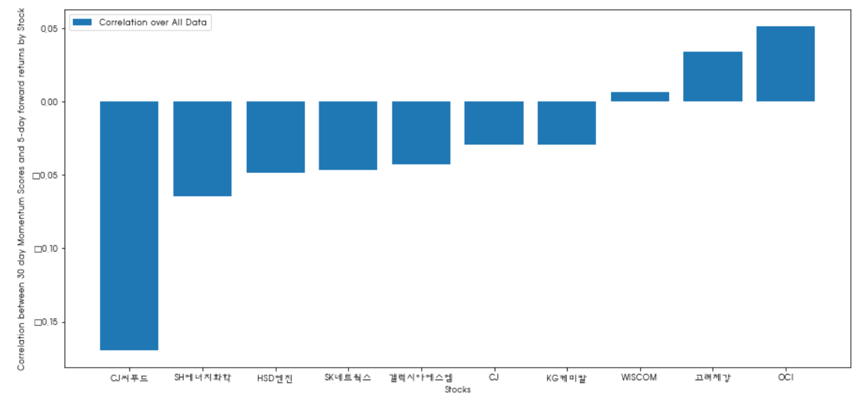
대부분의 주식의 모멘텀(30일)과 향후 수익률(5일)의 상관관계가 마이너스이다. 모멘텀 지표에 랭킹을 매김으로써 다음 한주를 예상해볼 수 있다.
높은 모멘텀 지표는 낮은 수익률 리턴을 예상할 수 있다.
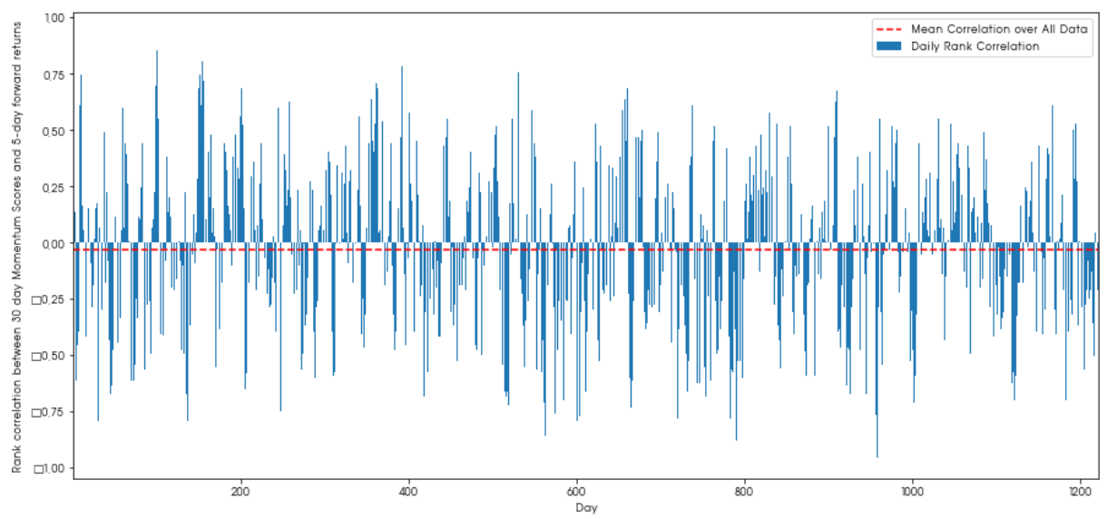
일별 상관관계
correl_scores = pd.DataFrame(index = returns.index.intersection(mscores.index), columns = ['Scores', 'pvalues'])
for i in correl_scores.index:
    score, pvalue = stats.spearmanr(mscores.loc[i], returns.loc[i])
    correl_scores['pvalues'].loc[i] = pvalue
    correl_scores['Scores'].loc[i] = score
correl_scores.dropna(inplace = True)
l = correl_scores.index.size
plt.figure(figsize=(15,7))
plt.bar(range(1,1+l),correl_scores['Scores'])
plt.hlines(np.mean(correl_scores['Scores']), 1,l+1, colors='r', linestyles='dashed')
plt.xlabel('Day')
plt.xlim((1, l+1))
plt.legend(['Mean Correlation over All Data', 'Daily Rank Correlation'])
plt.ylabel('Rank correlation between %s day Momentum Scores and %s-day forward returns'%(day,forward_return_day));
plt.show()
일별상관관계는 잡음이 많지만 평균치는 약간의 마이너스이다.
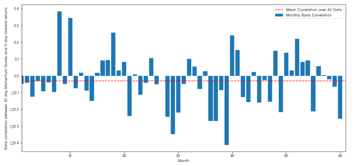
월별 상관관계
monthly_mean_correl =correl_scores['Scores'].astype(float).resample('M').mean()
plt.figure(figsize=(15,7))
plt.bar(range(1,len(monthly_mean_correl)+1), monthly_mean_correl)
plt.hlines(np.mean(monthly_mean_correl), 1,len(monthly_mean_correl)+1, colors='r', linestyles='dashed')
plt.xlabel('Month')
plt.xlim((1, len(monthly_mean_correl)+1))
plt.legend(['Mean Correlation over All Data', 'Monthly Rank Correlation'])
plt.ylabel('Rank correlation between %s day Momentum Scores and %s-day forward returns'%(day,forward_return_day));
plt.show()
월별데이텉 역시 약간의 잡음은 있디만 마이너스 상관관계를 갖음을 확인할 수 있다.
4. Basket 구성하기
주식별 예상 성과(Factor Values)에 따라 바스켓을 나눌수 있다. 해당 예에서 지정한 Factor Values는 모멘텀 지수이다.
모멘텀 지표에 따라 모든 주식의 순위를 매기고 그들을 그룹으로 나눈다면, 각 그룹의 평균 수익은 무엇입니까?
월별 Basket 평균 수익률 구하기
def compute_basket_returns(factor, forward_returns, number_of_baskets, index):

    data = pd.concat([factor.loc[index],forward_returns.loc[index]], axis=1)

    # Rank the equities on the factor values
    data.columns = ['Factor Value', 'Forward Returns']
    data.sort_values('Factor Value', inplace=True)

    # How many equities per basket
    equities_per_basket = np.floor(len(data.index) / number_of_baskets)
    basket_returns = np.zeros(number_of_baskets)

    # Compute the returns of each basket
    for i in range(number_of_baskets):
        start = i * equities_per_basket
        if i == number_of_baskets - 1:
            # Handle having a few extra in the last basket when our number of equities doesn't divide well
            end = len(data.index) - 1
        else:
            end = i * equities_per_basket + equities_per_basket
        # Actually compute the mean returns for each basket
        #s = data.index.iloc[start]
        #e = data.index.iloc[end]
        basket_returns[i] = data.iloc[int(start):int(end)]['Forward Returns'].mean()

    return basket_returns
다만, 이 데이터는 적정 기간에 대한 검증이 필요하다.
이제 바스켓별 수익률을 산출해보자. 바스켓수는 5개로 지정하였다.
number_of_baskets = 5
mean_basket_returns = np.zeros(number_of_baskets)
resampled_scores = mscores.astype(float).resample('2D').last()
resampled_prices = data.astype(float).resample('2D').last()
resampled_scores.dropna(inplace=True)
resampled_prices.dropna(inplace=True)
forward_returns = resampled_prices.shift(-1)/resampled_prices -1
forward_returns.dropna(inplace = True)

for m in forward_returns.index.intersection(resampled_scores.index):
    basket_returns = compute_basket_returns(resampled_scores, forward_returns, number_of_baskets, m)
    mean_basket_returns += basket_returns
mean_basket_returns /= l
print(mean_basket_returns)

# Plot the returns of each basket
plt.figure(figsize=(15,7))
plt.bar(range(number_of_baskets), mean_basket_returns)
plt.ylabel('Returns')
plt.xlabel('Basket')
plt.legend(['Returns of Each Basket'])
plt.show()

이제 바스켓을 통해 저성과가 예상되는 주식을 쉽게 구별해낼 수 있게 되었다.
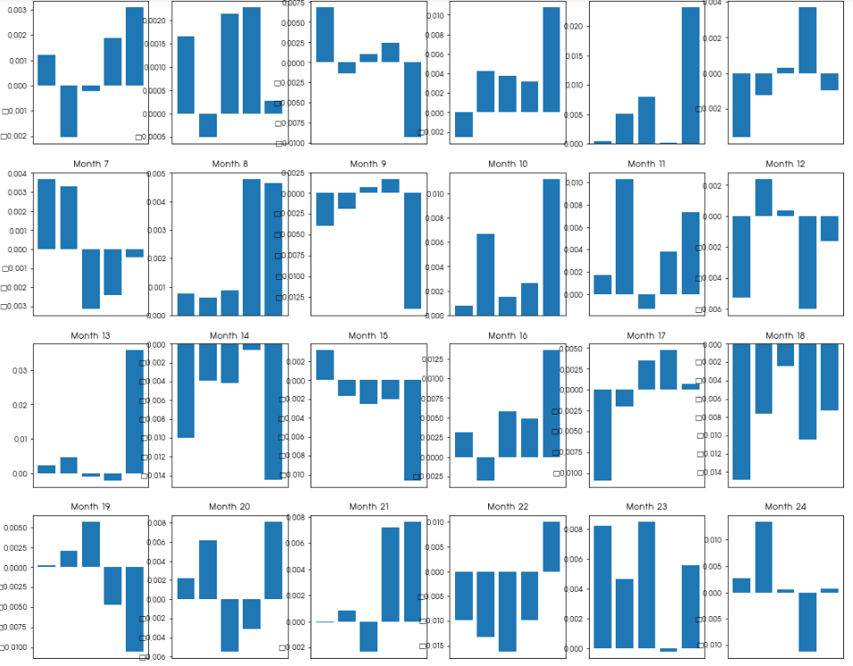
5. 스프레드 일관성 확인
모멘텀과 수익률의 상관관계를 활용한 전략은 단지, 과거 평균적인 관계입니다. 이것이 얼마나 일관성이 있는지를 파악해 봐야 한다. 아래 그래프는 최근 2년치를 확인해본 결과이다.
전략은 월별로 고성과 예상 주식 Basket을 매수하고 저성과 예상 주식 Basket을 매도하는 전략을 취한다.
이 전략의 성과는 편차가 있을 수 있다. 편차의 정도를 확인하여 모멘텀 지표가 Factor Values로서 가치가 있는지 살펴 본다.
total_months = mscores.resample('M').last().index
months_to_plot = 24  # 2년
monthly_index = total_months[-months_to_plot-1:]  # 초기 : [:months_to_plot+1], 최근 : [-months_to_plot-1:]
mean_basket_returns = np.zeros(number_of_baskets)
strategy_returns = pd.Series(index = monthly_index)
f, axarr = plt.subplots(int(monthly_index.size/6), 6,figsize=(18, 15))

for month in range(1, monthly_index.size):
    temp_returns = forward_returns.loc[monthly_index[month-1]:monthly_index[month]]
    temp_scores = resampled_scores.loc[monthly_index[month-1]:monthly_index[month]]

    for m in temp_returns.index.intersection(temp_scores.index):
        basket_returns = compute_basket_returns(temp_scores, temp_returns, number_of_baskets, m)
        mean_basket_returns += basket_returns

    strategy_returns[monthly_index[month-1]] = mean_basket_returns[ number_of_baskets-1] - mean_basket_returns[0]

    mean_basket_returns /= temp_returns.index.intersection(temp_scores.index).size

    r = int(np.floor((month-1) / 6))
    c = (month-1) % 6
    axarr[r, c].bar(range(number_of_baskets), mean_basket_returns)
    axarr[r, c].xaxis.set_visible(False)
    axarr[r, c].set_title('Month ' + str(month))

plt.show()
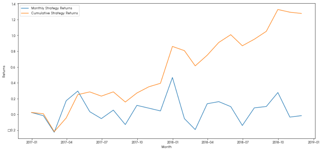
월별 수익률 추이
plt.figure(figsize=(15,7))
plt.plot(strategy_returns)
plt.ylabel('Returns')
plt.xlabel('Month')
plt.plot(strategy_returns.cumsum())
plt.legend(['Monthly Strategy Returns','Cumulative Strategy Returns'])
plt.show()
월별 플러스 수익률을 기록하고 있으며 누적수익률이 지속 증가하는 것을 확인할 수 있다.
마지막 Basket을 매수하고 매월 첫번째 Basket을 매도한 경우의 수익률 시뮬레이션 결과는 다음과 같다.
total_return = strategy_returns.sum()
ann_return = 100*((1 + total_return)**(12.0 /float(strategy_returns.index.size))-1)
print('Annual Returns: %.2f%%'%ann_return)
Annual Returns: 48.43%
6. Ranking Scheme
정확하고 바른 Ranking Scheme를 찾는것은 매우 중요하다.
또한 이 전략은 시점마다 유의성이 달라질 수 있어, 현상황에서 일관성이 어느정도 유지될지 파악하는 것도 중요하다.
Ranking Scheme를 설정하는 Tip은 아래와 같다.
Factor Values를 뭘로 사용할지 잘 판단해야 한다.
-
가격 기반 요인 (기술 지표) : 각 주식의
과거 가격에 대한 정보를 가져 와서 요인 가치를 생성하는 데 사용한다.
이동 평균 측정, 운동량 리본 또는 변동성 측정이 그 예이다. -
Reversion vs. Momentum : 일단 방향으로 움직이면 가격이 계속 그렇게 될 것이라는 점에 유의해야 한다.
그 반대의 요인들도 있다. 둘 다 서로 다른 시간대와 자산에 대한 유효한 모델이며 기본 동작이 기세 또는 반전 기반인지 여부를 조사하는 것이 중요하다. -
Fundamental Factors (가치 기반) : P.E 비율, 배당금 등과 같은 기본 가치의 조합을 사용한다.
근본적인 가치는 회사에 대한 실제 사실에 연결된 정보를 포함하므로 여러면에서 가격보다 더 강력 할 수 있다.
어떠한 요인이든 일관성이 희석되는 수명을 갖기 때문에, 얼마나 유효한지 지속 검증이 필요하며 어떤 새로운 요인을 사용할수 있는지 지속 발굴하려는 노력이 중요하다.
Reference
https://medium.com/auquan/long-short-equity-trading-strategy-daa41d00a036